Background
There are two types of analyses in statistics that are well known. One is frequentist analysis - confidence intervals, p values, etc. Another is bayesian analysis. Bayesians use their prior beliefs in combination with the data to come up with probability distributions (curves that integrate to 1, and show relative probabilities.). Most technical people know about frequentist analysis, and have heard of p values and such. I'm going to introduce you to bayesian analysis. For best results, I suggest that you follow along with paper and pencil.
Introduction
Barry Bonds is a pretty great baseball player. What if, as a curious statisticians, you want to find out the probability \(\theta\) that he hits a home run on any given at-bat? What you have is data - a number of at-bats and whether Bonds has hit a home run for each. That's great for when you know \(\theta\), because you can tell me how likely it was that the data happened. We call this the likelihood function, and it's denoted \(f(\text{data | } \theta) = \text{how likely the data happened given the probability } \theta\). This means that you have some known \(\theta\) and, using f, you can find out how likely the data is. The problem is that we have the reverse. We know the data, but we don't know what Bonds' home-run hitting probability is.
It turns out that we can use Bayes' theorem to switch the conditions of our likelihood, \(f\). Bayes theorem is defined as:
$$ \begin{align*} P(A\text{ | }B) &= \frac{P(B\text{ | }A) * P(A)}{P(B)} \end{align*} $$Let's recap. I have \(f(\text{data | }\theta)\), I want a function with the conditions swapped, let's call it \(g(\theta\text{ | data})\). Let's try plugging it into Bayes' Theorem.
$$ \begin{align*} g(\theta\text{ | data}) &= \frac{f(\text{data | }\theta)*\pi(\theta)}{\text{probability of data}} \end{align*} $$We're clearly missing two parts. What is \(\pi(\theta)\)? How do we define the probability of the data?
Prior distributions
It turns out that \(\pi(\theta)\) is a crucial part of Bayesian analysis - it's called the prior distribution. Remember that I said that Bayesians use their prior beliefs in combination with the data? \(\pi(\theta)\) are those prior beliefs. Maybe, for example, I thought that Barry Bonds' home run hitting percentage was about 10%. I'd make a statistical distribution around that value: say, a Beta distribution with \(\alpha = 49, \beta = 431\). Where did I get those numbers? I just made them up. This is part of the controversy of the Bayesian method.
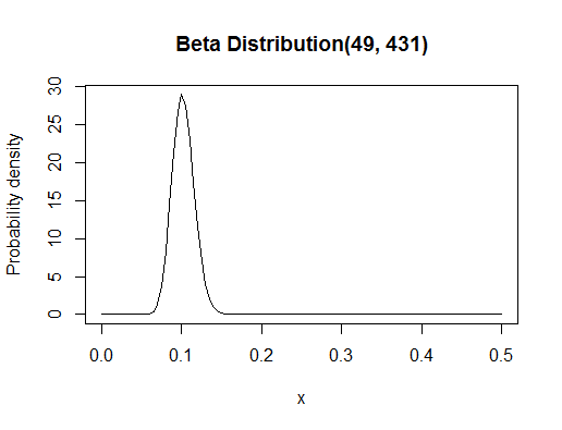
You might be confused about what a Beta distribution is. Statistical distributions like the Beta distribution are functions that have configurable settings. The Beta distribution has two settings, \(\alpha\) and \(\beta\). Setting them gives you a particular curve - in this case, it looks like:

Notice that with this distribution, I'm showing both my expectation, as you can see from the "highest density" part being around 0.1, and also my uncertainty, which you can see by the spread. If I was really unsure, the curve would be very flat. I'm using a distribution as my prior belief because it can represent my beliefs fully.
Probability of the Data?
Remember when I said that "Bayesians use their prior beliefs in combination with the data to come up with probability distributions?" The last two words are key: probability distribution. One of the key features of a probability distribution is that it integrates to 1. Thus, the denominator in our Bayes' theorem equation is going to have to be the area under our new probability distribution on \(\theta\). How do we get the area? Integration. It is well known that the Beta distribution is bounded, with domain [0, 1]. Thus, the denominator will be \(\int_0^1f(\text{data | }\theta)*\pi(\theta)d\theta\), and our full equation to find \(g\) will be:
$$ \begin{align*} g(\theta\text{ | data}) &= \frac{f(\text{data | }\theta)*\pi(\theta)}{\int_0^1f(\text{data | }\theta)*\pi(\theta)d\theta} \end{align*} $$Stare at this for a while until you can explain to yourself, out loud, every part. Then take a deep breath, and let's write in the numbers.
Definitions
Notice that the data we were given, at-bats and whether they were home runs or not, follow what we call a Binomial Distribution. Thus, we're going to say that \(f(\text{data | }\theta)\) follows a Binomial distribution. A Binomial distribution is meant to represent the number of successes in a sequence of Bernoulli trials. A Bernoulli trial is a test that results in either success or failure. The settings of this Binomial distribution are the number of at-bats, and the probability of Barry Bonds hitting a home run. After configuring those settings, the Binomial distribution is a function where you put in the number of home runs, \(y\), and you get out the probability of \(y\) home runs happening.
A note about how we will represent the data: in this case, the at-bat is the test, the home run is the success, and the non-home run is a failure. We can thus represent our data as a string of 0s and 1s. Summing the 1s gives us the total number of home runs, let's call it \(y\). Subtracting \(y\) from the total number of numbers, \(n\) (e.g. 00101 would be 5 numbers), gives us the total number of failures.
I'll just hand the data to you. \(y = 73, n = 476, n - y = 403\).
Mathematically, a Binomial distribution function (which is our likelihood function) is defined as:
$$ \begin{align*} f(\text{data | }\theta) &= \binom{n}{y}\theta^y(1 - \theta)^{n - y} \end{align*} $$Remember that \(n, \theta\) are the settings, meaning that \(n, \theta\) are constant in the above equation. All we're changing is \(y\). This is why the distribution is still a two dimensional curve.
The Beta distribution is a curve that is bounded by [0, 1], so it's good for representing probabilities. You could say it's a probability distribution on probabilities. It's settings are \(\alpha, \beta\) and you put in a number between 0 and 1, and you get out a number between 0 and 1, which represents the probability of your probability. It's confusing, I know. Mathematically, it's defined as:
$$\pi(\theta) = \frac{\Gamma(\alpha + \beta)}{\Gamma(\alpha)\Gamma(\beta)}\theta^{\alpha - 1}(1 - \theta)^{\beta - 1}$$Remember that \(\alpha, \beta\) are constant! You put in \(\theta\) here, and you get out the probability of \(\theta\).
Posterior Distribution
The theory stops here. Leave if you want. Continue if you want to see this Barry Bonds example through.
We're going to plug in our mathematical definitions into our Bayes' theorem equation, and we're going to do a ton of algebra, and then we're going to end up with something surprising. Here we go.
To keep things a little shorter, I'm going to write \(y\) instead of "data". I'm also going to write "a" instead of \(\alpha\) and "b" instead of \(\beta\), because Bayesians usually save the Greek for unknown parameters, and we set a and b ourselves, so they are known.
$$\begin{align*} \pi(\theta | y) &= \frac{f(y\text{ | }\theta)\pi(\theta\text{ | }a, b)}{\int_0^1f(y\text{ | }\theta)\pi(\theta\text{ | }a, b)d\theta}\\[2ex] &= \Pi_{i=1}^{n}\frac{\binom{n_i}{y_i}\theta^{y_i}(1 - \theta)^{n_i - y_i})\frac{\Gamma(a + b)}{\Gamma(a)\Gamma(b)}\theta^{a - 1}(1 - \theta)^{b - 1}}{\int_0^1\binom{n_i}{y_i}(\theta^*)^{y_i}(1 - \theta^*)^{n_i - y_i}\frac{\Gamma(a + b)}{\Gamma(a)\Gamma(b)}(\theta^*)^{a - 1}(1 - \theta^*)^{b - 1}d\theta}\\[2ex] &= \frac{\Pi_{i=1}^{n}(\binom{n_i}{y_i})\frac{\Gamma(a + b)}{\Gamma(a)\Gamma(b)}\theta^{\Sigma_{i=1}^{n}y_i}(1 - \theta)^{\Sigma_{i=1}^{n}n_i - y_i})\theta^{a - 1}(1 - \theta)^{b - 1}}{\Pi_{i=1}^{n}(\binom{n_i}{y_i})\frac{\Gamma(a + b)}{\Gamma(a)\Gamma(b)}\int_0^1(\theta^*)^{\Sigma_{i=1}^{n}y_i}(1 - \theta^*)^{\Sigma_{i=1}^{n}n_i - y_i}(\theta^*)^{a - 1}(1 - \theta^*)^{b - 1}d\theta}\\[2ex] &\text{Note that the combinations and gamma terms cancel,}\\ &= \frac{\theta^{\Sigma_{i=1}^{n}(y_i) + a - 1}(1 - \theta)^{\Sigma_{i=1}^{n}(n_i - y_i) + b - 1}}{\frac{\Gamma(\Sigma_{i=1}^{n}(y_i) + a)\Gamma(\Sigma_{i=1}^{n}(n_i - y_i) + b)}{\Gamma(\Sigma_{i=1}^{n}(y_i) + a + \Sigma_{i=1}^{n}(n_i - y_i) + b)}\int_0^1\frac{\Gamma(\Sigma_{i=1}^{n}(y_i) + a + \Sigma_{i=1}^{n}(n_i - y_i) + b)}{\Gamma(\Sigma_{i=1}^{n}(y_i) + a)\Gamma(\Sigma_{i=1}^{n}(n_i - y_i) + b)}(\theta^*)^{\Sigma_{i=1}^{n}y_i + a - 1}(1 - \theta^*)^{\Sigma_{i=1}^{n}(n_i - y_i) + b - 1}d\theta}\\[2ex] &\text{Note that the integral term now goes to 1, by definition}\\[2ex] &= \frac{\Gamma(\Sigma_{i=1}^{n}(y_i) + a + \Sigma_{i=1}^{n}(n_i - y_i) + b)}{\Gamma(\Sigma_{i=1}^{n}(y_i) + a)\Gamma(\Sigma_{i=1}^{n}(n_i - y_i) + b)}\theta^{\Sigma_{i=1}^{n}(y_i) + a - 1}(1 - \theta)^{\Sigma_{i=1}^{n}(n_i - y_i) + b - 1}\\[2ex] \pi(\theta | y) &\sim \text{Beta}(a + \Sigma_{i=1}^{n}(y_i), b + \Sigma_{i=1}^{n}(n_i - y_i)) \end{align*} $$This may surprise you, and it only happens rarely. It turns out that if you combine the Beta distribution and the Binomial distribution, you get a another Beta distribution with different, but related settings. Our posterior distribution is that new Beta distribution. You can see from the formulas that the posterior distribution's settings are found by adding the total # of home runs to a, and the total # of at-bats - total # of home runs to b.
Results
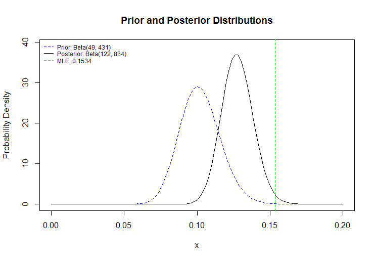
Let's plug in the specific numbers we mentioned earlier. a = 49, b = 431, y = 73, n = 476, n - y = 403. Our posterior distribution has parameters \(a^\prime = 49 + 73 -> a^\prime = \boxed{122}, b^\prime = 431 + (476 - 73) -> b^\prime = \boxed{834}\). Here's what we get:

The green line is something I didn't tell you about - it's what frequentist statisticians would come up with as Barry Bonds' true home-run-hitting average. Notice that it's not a distribution, and it's not a probability either - it's the value of \(\theta\) that, had you plugged it into \(f\), would have produced the highest value. In other words, it's the value of \(\theta\) that makes our observed data the likeliest to happen, and it's called the Maximum Likelihood Estimator. Meanwhile, Bayesian analysis has given us a whole distribution which both shows what we expect (the highest part of the distribution, or expected value), as well as the uncertainty that we have, shown by the spread of the distribution. The prior distribution on the left shows that we expected Bonds to do worse than he actually did, so the posterior dragged the expected value up and tightened the spread because, with more data, we're now more sure about Bonds' home run hitting average.