Prerequisites
There's a lot of statistical jargon thrown around in here. I recommend, if you're interested in really understanding what this algorithm buys you, researching what statistical distributions and probability densities are, how to sample from a known distribution, and perhaps even rejection or importance sampling. Although, without knowing those concepts, you could probably still get by.
Background
Let's suppose you have a distribution from which you want to sample. Unfortunately, there is no easy way to find its density analytically, since sometimes the normalizing constant is really hard to calculate. However, we can use a technique called Markov Chain Monte Carlo sampling to get something close. Metropolis-Hastings is one such technique. MH buys you the density of an unnormalized target distribution.
A markov chain is simply a list of numbers, where the number at index i is only dependent on the number at index i - 1. This means we have a list of slightly dependent draws. The "slightly dependent" part is the tradeoff for getting what we want - a set of samples from the target distribution (so called kernel/target distribution). But it turns out that the markov chain we're talking about is ergodic. Being ergodic means that you satisfy three properties - you're aperiodic (there's no cycle), irreducible (there's a way to go from one state to any other state in the system, albeit it might take more than 1 step), and positive recurrent, so it's expected that the return time to some state \(i\) is finite (a.k.a, you can come back to states within reasonable time). Most of the Markov chains used in Bayesian Statistics are ergodic.
Being ergodic buys us the ability to ignore the slight dependence between draws. More specifically, the Ergodic Theorem says that for an ergodic Markov chain with expected value less than infinity, with probability 1 or absolute certainty,
$$\frac{1}{M}\Sigma_{i=1}^Mg(\theta_i) \rightarrow \int_{\Theta}g(\theta)\pi(\theta)d\theta$$Each symbol means something. \(M\) is the number of values in the Markov chain, \(\pi\) is the target distribution we want draws from, \(\theta\) represents the values of the Markov chain, such that \(\theta_1, \theta_2\) refer to the first and second values of the chain, and \(g\), I believe, refers to the probability density of a particular \(\theta\). Write me a note if you'd like to clarify.
All this means is that we're good to go mathematically if we draw many Markov chain values from our target distribution.
Algorithm
There are some ingredients to this algorithm. We need a chain of values with some arbitrary starting value, and a way to dictate what the next value in the chain will be. What dictates the next value is called the candidate distribution. It can be anything, really, but most often people pick symmetric distributions as the candidate distribution. If the main mass of the target distribution is grouped in some asymmetric way, using an asymmetric candidate distribution might help performance, but this is is a rarer case. For simplicity's sake, and because hand-tuning the asymmetric candidate distribution is hard, we'll use a very simple candidate distribution - a uniform distribution between x - 3 and x + 3. x will be the current value of the markov chain. Notice that this is where we see that the draws are slightly dependent.
For our target distribution, we'll use a modified T distribution that would ordinarily be hard to find the normalizing constant for. We'll say that the target distribution is \(\frac{1 + (x - 10)^2}{3})^{-2}\)
Once we draw a candidate value from the candidate distribution, there's a probability of accepting that value as the next value, which is \(\frac{\text{Target Distribution Density at new value}}{\text{Target Distribution Density at previous value}}\). This tells us how likely it is to get to that next value, and we generate a random number between 0 and 1 to determine if we actually jump there or not. If our random probability is less than the acceptance probability, we take the draw. If not, we keep the old value. This is a critical feature of the Metropolis-Hastings algorithm.
Intuitively, what's going on is that we're placing a little point somewhere, arbitrarily onto the space. From that point, we make little jumps in some directions, deciding if it's worthwhile to make the jump. After many, many jumps, with the probability of each jump dictated by the target distribution, the density of all the jumps/draws we did will be approximately the target distribution we were trying to find.
"But wait", you say, "how could we possibly be sampling from the distribution if the first point is arbitrary?" One popular thing to do is to "burn out" the first 100 draws or so, since we know they could be arbitrary. After taking a million draws, the first 100 are inconsequential.
Here's some R code for you to solidify the concept.
ALPHA = 3
mh = function (n, target, STARTING_VALUE = 3, burnIn = 10, candidate = function (x) { runif(1, x - ALPHA, x + ALPHA) }) {
  xs = rep(STARTING_VALUE, n)
  for (i in 2:n) {
    y = candidate(xs[i - 1])
    acceptance = target(y) / target(xs[i - 1])
    xs[i] = if (runif(1) < acceptance) y else xs[i - 1]
  }
  xs[burnIn:length(xs)]
}

# Example call to draw from our target distribution
draws = mh(n = 100000, target = function (x) { return(((1 + (x - 10)^2)/3)^(-2)) }, burnIn = 100)
Notice that the acceptance percentage depends on the spread of the candidate distribution. For this particular example, I picked a candidate distribution that can select any x value 3 away from the current value. This yields an acceptance percentage of about 37%. There's no right answer for the acceptance percentage, but generally I would say that less than 20% is too inefficient and greater than 50% is too relaxed. Too strict or loose of an acceptance policy could mean, for example, that the most concentrated part of the target distribution will be blown out of proportion by our MCMC algorithm.
Results (with trace plot)
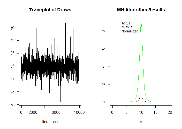
Empirical mean and standard deviation were 9.991816, and 0.8878 respectively. Quantiles:
  2.5%    25%    50%    75%  97.5%
 8.247  9.527  9.983 10.424 11.721
Notice that the dotted red and black lines are essentially coincidental. This is good news. The trace plot shows that the draws were pretty consistent and the MCMC algorithm was doing its job. A sectioned trace plot, were there are groups of draws in far away places, would be bad. Also note that 100 entries were burned off the chain. Another way to reduce the length of the chain is the "thin it out" by removing every nth draw. I didn't do that here.
Diagnostics & Reports
When using the MH algorithm, it's important to make sure you and others know:
- Target distribution
- Candidate distribution
- Starting value
- # burned off
- Thinning rate (3 means every third entry was removed)
- Empirical mean and standard deviation
- Trace plot
There are other good convergence and diagnostic statistics, but I think this is a good start.
Questions & Answers
1. What if I have a starting value outside my target distribution?
Hand-tune your algorithm so that the startig value is not outside your target distribution. It turns out that most questions I had when I started learning how to do this had to do with specific values and random events. However, it turns out that it's common practice to hand-tune your Metropolis-Hastings algorithm. There are adaptive MH algorithms, but often they're cost more than they're worth.
2. Why not rejection sampling?
Metropolis Hastings is faster, especially for oddly shaped distributions. If the distribution you'd like to sample from is uniform or fits under a known distribution nicely, then sure, use rejection/importance sampling.