Slice sampling is a form of Markov Chain Monte Carlo sampling, like the Metropolis Hastings. To see why this works (ergodic theorem), read the Metropolis Hastings writeup.
In rejection sampling, there's a probability of rejection. In slice sampling, there isn't. It's simply because of the algorithm that slice sampling employs:
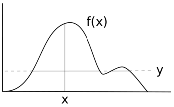
- Choose a random starting value of x, let's call it x1
- Uniformly sample on interval [0, f(x1)], let's call it a
- Here's the tricky part - imagine a horizontal line at y = a. Figure out all the line segments under the curve.
- From all the line segments, draw a value of x uniformly.
- Repeat from step 2 until you have as many draws as you want.
Advantages
- Easier to implement than Metropolis Hastings
- Faster than Rejection sampling
- The step-size feature of MH is tough to get right, and is constant. Slice-sampling auto-adjusts the step size for you.
- In the cases of slow sampling because of the shape of the distribution (the bigger the x interval, the slower it is to find the roots of the intersections), you can fit slice sampling with an ellipcal curve for say, Guassian priors.
Disadvantages
- Probably slower than Metropolis Hastings.
- Finding the roots of the intersection between horizontal line and distribution is pretty tricky. See the implementation below for a very naive example.
Code
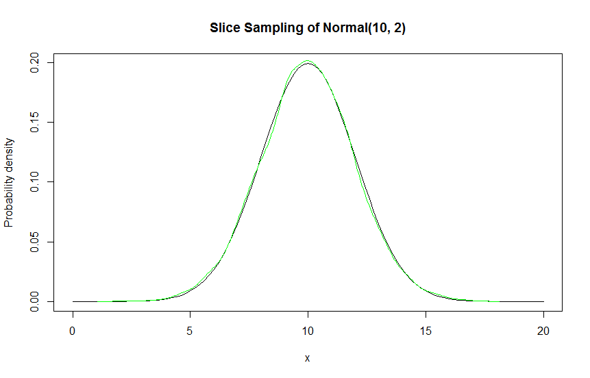
Here's a code sample in R. This implements slice sampling of a normal distribution with mean 10 and standard deviation 2. I used an x interval of 0 to 20, with 0.1 root finding step size.
The way I find the roots is very naive. I step through the interval, looking for sign differences - if I find one, I use R uniroot to locate the root. I then iterate through each root and take the midpoint, checking if it's under the curve to detect a valid line segment. Then, I distribute probabilities to the line segments, sampling one segment. Then, I uniformly select an x from the sampled line segment.
sliceSample = function (n, f, x.interval = c(0, 1), root.accuracy = 0.01) {
  # n is the number of points wanted
  # f is the target distribution
  # x.interval is the A,B range of x values possible.

  pts = vector("numeric", n)  # This vector will hold our points.
  x = runif(1, x.interval[1], x.interval[2]) # Take a random starting x value.

  for (i in 1:n) {
    pts[i] = x
    y = runif(1, 0, f(x))    # Take a random y value

    # Imagine a horizontal line across the distribution.
    # Find intersections across that line.
    fshift = function (x) { f(x) - y }
    roots = c()
    for (j in seq(x.interval[1], x.interval[2] - root.accuracy, by = root.accuracy)) {
      if ((fshift(j) < 0) != (fshift(j + root.accuracy) < 0)) {
        # Signs don't match, so we have a root.
        root = uniroot(fshift, c(j, j + root.accuracy))$root
        roots = c(roots, root)
      }
    }
    # Include the endpoints of the interval.
    roots = c(x.interval[1], roots, x.interval[2])

    # Divide intersections into line segments.
    segments = matrix(ncol = 2)
    for (j in 1:(length(roots) - 1)) {
      midpoint = (roots[j + 1] + roots[j]) / 2.0
      if (f(midpoint) > y) {
        # Since this line segment is under the curve, add it to segments.
        segments = rbind(segments, c(roots[j], roots[j + 1]))
      }
    }

    # Uniformly sample next x from segments
    # Assign each segment a probability, then unif based on those probabilities.
    # This is a bit of a hack because segments first row is NA, NA
    # Yet, subsetting it runs the risk of reducing the matrix to a vector in special case.
    total = sum(sapply(2:nrow(segments), function (i) {
      segments[i, 2] - segments[i, 1]
    }))
    probs = sapply(2:nrow(segments), function (i) {
      (segments[i, 2] - segments[i, 1]) / total
    })

    # Assign probabilities to each line segment based on how long it is
    # Select a line segment by index (named seg)
    p = runif(1, 0, 1)
    selectSegment = function (x, i) {
      if (p < x) return(i)
      else return(selectSegment(x + probs[i + 1], i + 1))
    }
    seg = selectSegment(probs[1], 1)

    # Uniformly sample new x value
    x = runif(1, segments[seg + 1, 1], segments[seg + 1, 2])
  }

  return(pts)
}

target = function (x) { dnorm(x, 10, 2) }
points = sliceSample(n = 10000, target, x.interval=c(0, 20), root.accuracy = 0.1)
curve(target, from = 0, to = 20, ylab="Probability density", main="Slice Sampling of Normal(10, 2)")
lines(density(points), col="green")